
The Limitations of Mean Squared Error in Physical Forecasting
Mean Squared Error (MSE), a ubiquitous metric in machine learning, provides a seemingly straightforward measure of prediction accuracy. It penalizes larger errors more heavily than smaller ones, making it a popular choice for regression tasks. However, when forecasting physical signals—think sensor readings, weather patterns, or industrial process parameters—MSE can be profoundly misleading. This is the central thesis of the second installment in a series exploring probabilistic forecasting for these complex domains.
The core issue lies in MSE's inability to capture the nuances of uncertainty inherent in physical systems. Physical signals are often stochastic, influenced by myriad unobserved factors and exhibiting complex temporal dependencies. A model that consistently underestimates or overestimates a signal, but with low variance, might appear superior to one that is more accurate on average but exhibits higher variance. MSE treats all errors equally in terms of their impact on the metric, regardless of whether they represent a predictable deviation or a true, irreducible uncertainty.
Furthermore, MSE is a point-estimate metric. It evaluates a single predicted value against a single true value. In many physical forecasting scenarios, particularly those involving time series, we are not just interested in the most likely future value, but also in the range of plausible future values. This is where probabilistic forecasting—which aims to predict a probability distribution over future outcomes—becomes crucial. Without considering the uncertainty, a model optimized solely for MSE might produce brittle predictions that fail catastrophically when faced with unexpected but statistically likely events.
Autoregressive Rollout: Extending Forecast Horizons
A common challenge in time series forecasting is extending predictions beyond the immediate future. Autoregressive models, by definition, use past values to predict future ones. When forecasting multiple steps ahead, a technique known as autoregressive rollout becomes essential. In this method, the model's own previous predictions are fed back as inputs for subsequent predictions. For instance, to predict t+2, the model uses the predicted value at t+1 as an input, along with historical data up to t.
The problem with this approach, especially when combined with an MSE-optimized model, is the compounding of errors. Each step into the future introduces a new layer of potential inaccuracy. If the prediction at t+1 is slightly off, that error is propagated and amplified when predicting t+2. This effect can lead to forecasts that diverge significantly from reality as the forecast horizon increases, rendering the MSE metric increasingly unrepresentative of actual performance over longer periods. A model that achieves low MSE for a one-step-ahead forecast might produce wildly inaccurate multi-step forecasts due to this error propagation.
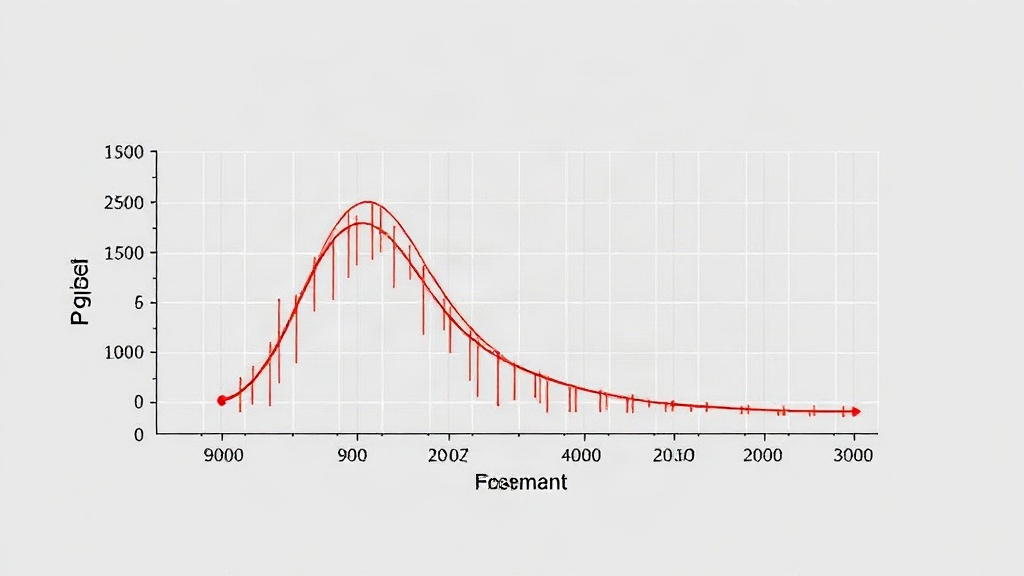
This compounding effect highlights why focusing solely on MSE is problematic. It doesn't account for the model's confidence or the potential for divergence over time. A more robust evaluation would consider how the uncertainty band around the predictions grows with each autoregressive step.
Uncertainty Propagation: Quantifying Forecast Risk
Probabilistic forecasting aims to address the limitations of point estimates by providing a distribution of possible outcomes. This distribution inherently captures the uncertainty associated with the forecast. However, the process of generating these probabilistic forecasts, especially through autoregressive rollout, requires careful consideration of how uncertainty propagates. Uncertainty propagation is the study of how uncertainty in measurements or model inputs affects the uncertainty in outputs.
In the context of autoregressive forecasting, each prediction step can introduce or amplify uncertainty. If a model predicts a value at t+1 with a wide confidence interval, feeding that entire interval (or a representation of it) into the next step can lead to an even wider interval at t+2. Techniques for managing uncertainty propagation include Monte Carlo dropout, Bayesian neural networks, or ensemble methods, where multiple models or multiple forward passes with dropout can generate a distribution of outputs.
The critical insight here is that the *growth* of uncertainty over the forecast horizon is as important as the accuracy of the central prediction. A model that shows a rapidly widening uncertainty band might be signaling that its predictions become unreliable very quickly. Evaluating this propagation is key. Metrics that consider the width and shape of the predicted distribution, such as the Continuous Ranked Probability Score (CRPS) or the Negative Log-Likelihood (NLL), are often more appropriate than MSE for probabilistic forecasts. These metrics directly assess the quality of the entire predicted distribution, not just a single point.
What remains unaddressed by simple MSE is the model's ability to signal when it is