The Core Idea: A Two-Step Process
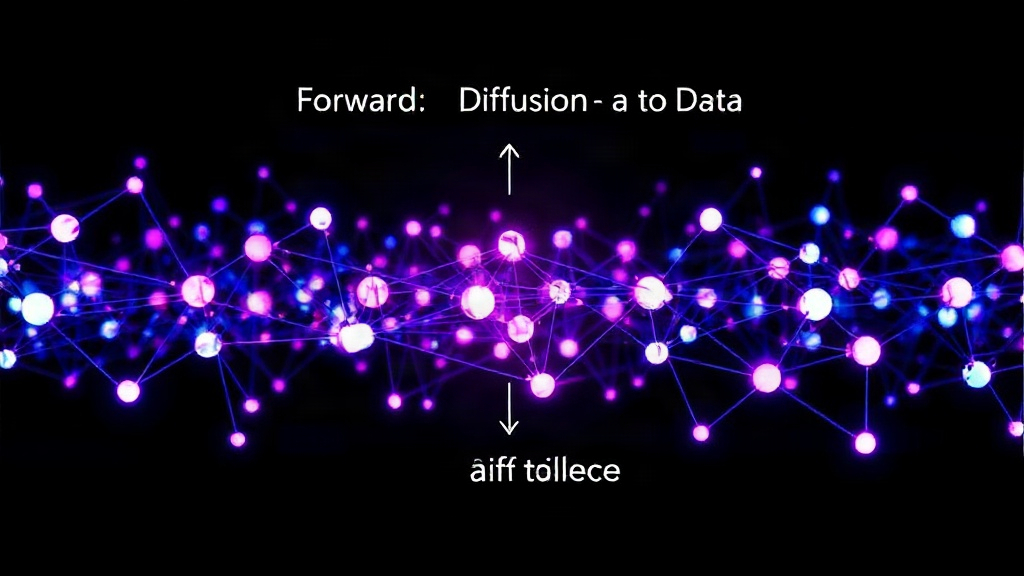
Diffusion models tackle the challenge of generating complex data, like high-resolution images, not by attempting a direct, one-shot solution. Instead, they employ a clever two-stage approach: a forward diffusion process and a learned reverse diffusion process. The forward process is designed to systematically destroy information in real data by gradually adding Gaussian noise over a series of discrete timesteps. This transforms a structured data sample into pure noise. The model's task is then to learn the reverse of this process – to start from random noise and, step-by-step, remove the noise to reconstruct a plausible data sample.
Think of it like this: imagine you have a perfectly clear photograph. The forward process is like slowly blurring it, adding more and more static, until it's just a grainy mess. The reverse process is learning how to take that grainy mess and, with precise steps, bring back the clarity to reveal the original photo, or a new one that looks just as real. This decomposition turns a seemingly intractable problem of generating complex distributions into a series of smaller, more manageable prediction tasks.
Formalizing the Forward Diffusion
Mathematically, the forward diffusion process can be defined as a Markov chain. At each timestep $t$, the data $x_t$ is obtained by adding a small amount of Gaussian noise to the data from the previous timestep $x_{t-1}$. This is typically expressed as:
$$x_t = \sqrt{1 - \beta_t} x_{t-1} + \sqrt{\beta_t} \epsilon_{t-1}$$
where $\epsilon_{t-1}$ is a standard Gaussian random variable, and $\beta_t$ is a small variance schedule that controls the amount of noise added at each step. As $t$ increases, $x_t$ progressively loses its structure and approaches a standard Gaussian distribution. Crucially, this forward process is fixed and requires no learning; it’s a predefined mathematical operation. The total number of diffusion steps, often denoted as $T$, is typically large, ranging from hundreds to thousands, ensuring that by step $T$, the original data $x_0$ is effectively indistinguishable from pure noise $x_T \sim \mathcal{N}(0, I)$.
Learning the Reverse: Noise Prediction
The real power of diffusion models lies in learning the reverse process. The goal is to predict the noise that was added at each step $t$ to get from $x_{t-1}$ to $x_t$. If the model can accurately predict the noise $\epsilon$ added at timestep $t$ when given the noisy data $x_t$, it can then reverse the step. The reverse transition can be approximated as:
$$x_{t-1} = \frac{1}{\sqrt{1 - \beta_t}} \left( x_t - \frac{\beta_t}{\sqrt{1 - \bar{\beta}_t}} \epsilon \right) + \sigma_t z$$
where $\bar{\beta}_t$ is the cumulative product of $\beta_i$ up to $t$, $z$ is a standard Gaussian variable, and $\sigma_t$ is a variance term. A common simplification, particularly in models like DDPM (Denoising Diffusion Probabilistic Models), is to train a neural network (often a U-Net architecture for image data) to directly predict the noise $\epsilon_t$ that was added to $x_0$ to produce $x_t$. This prediction is conditioned on the noisy data $x_t$ and the current timestep $t$.
The training objective is to minimize the difference between the actual noise added and the noise predicted by the network. This is often formulated as minimizing the mean squared error:
$$L = \mathbb{E}_{t \sim [1, T], x_0 \sim q(x_0), \epsilon \sim \mathcal{N}(0, I)} \left[ \left|\left| \epsilon - \epsilon_\theta(x_t, t) \right\|\right|^2 \right]$$
Here, $\epsilon_\theta(x_t, t)$ is the noise predicted by the neural network parameterized by $\theta$. By training on many data samples and various noise levels, the network learns to denoise effectively across the entire spectrum of corruption.
Generation: Sampling from Noise
Once the reverse process is learned, generating new data is straightforward. We start with a sample of pure Gaussian noise $x_T$. Then, we iteratively apply the learned reverse transition, using the trained network to predict the noise at each step and subtract it to move to a less noisy state $x_{t-1}$, until we reach $x_0$. This iterative denoising process, guided by the learned noise predictions, yields a generated sample that should resemble the data distribution the model was trained on.
The beauty of this approach is its flexibility. By controlling the number of steps and the noise schedule, one can influence the quality and diversity of generated samples. Furthermore, conditional diffusion models can incorporate additional information, such as text prompts or class labels, to guide the generation process, leading to powerful text-to-image or class-conditional image synthesis capabilities.
Why This Approach Works
The success of diffusion models stems from several factors. Firstly, they avoid the mode collapse issues that can plague other generative models like GANs, as they are trained to model the entire data distribution rather than just finding adversarial equilibria. Secondly, the step-by-step denoising process is inherently stable and allows for high-fidelity generation. The gradual refinement from noise to data mirrors how humans might imagine or construct complex concepts, starting from a vague idea and adding detail. This makes the learning problem more tractable for the neural network. The ability to turn a hard, high-dimensional generation problem into a sequence of simpler, localized denoising steps is the foundational insight that makes diffusion models so effective.