The Challenge of Scale: Why Exact Nearest Neighbor Search Fails
At its core, any system performing semantic operations—whether it's a Retrieval-Augmented Generation (RAG) pipeline, a recommendation engine, image search, or duplicate detection—relies on a single fundamental operation: given a specific vector, find the closest vectors from a massive dataset. These vectors, known as embeddings, are numerical representations, typically consisting of a few hundred to a couple of thousand numbers each. "Closest" in this context means closest in meaning or semantic similarity.
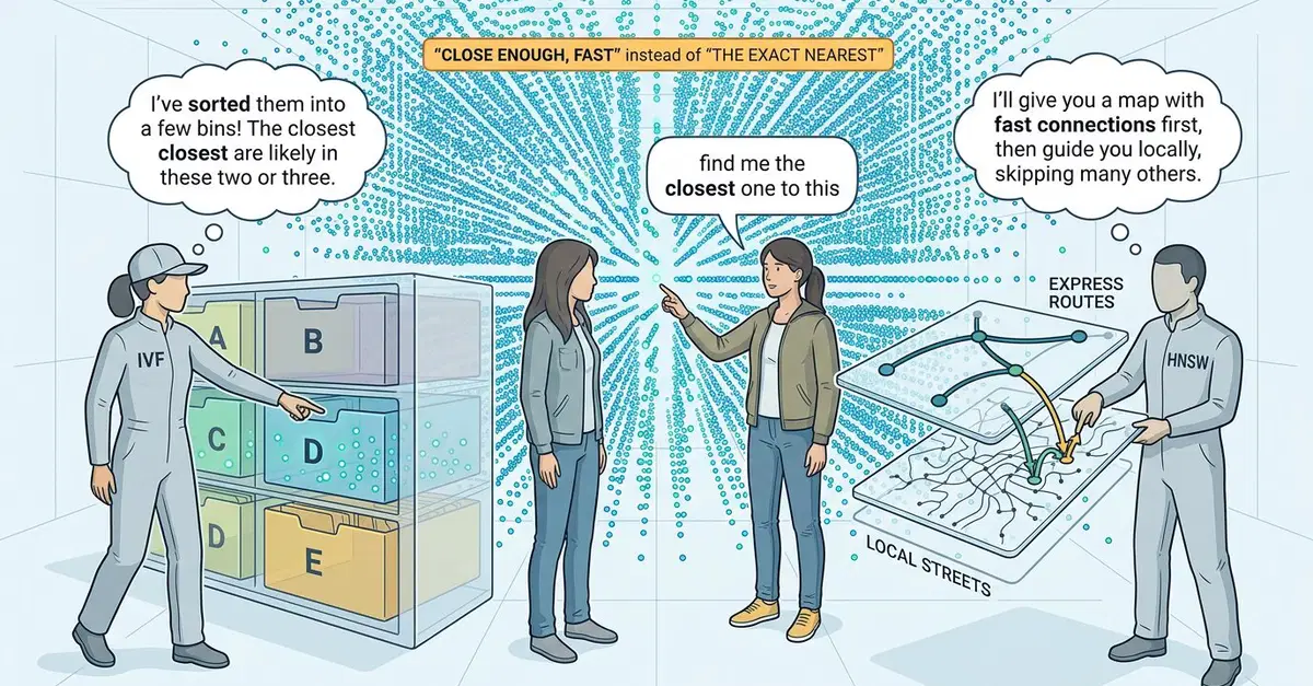
One might assume that a system would either linearly scan every single vector in the database (which is accurate but prohibitively slow for millions or billions of vectors) or employ a sophisticated tree-like structure to directly pinpoint the answer. The reality is that neither of these approaches is typically used. Instead, vector search systems deliberately settle for finding the approximately closest vectors. This compromise is the very foundation that makes vector search fast enough to be practical. Two algorithms, Inverted File Index (IVF) and Hierarchical Navigable Small Worlds (HNSW), handle the bulk of this work across popular vector databases and libraries like pgvector, Qdrant, and FAISS. Understanding what these algorithms actually do under the hood is crucial for selecting the right approach for your specific needs.
The immediate question for anyone encountering this is: why approximation? If we can find the exact nearest neighbors, why wouldn't we? The answer lies in the computational complexity. For a dataset of N vectors, each with D dimensions, finding the exact nearest neighbor requires computing the distance between the query vector and every other vector in the dataset. This scales linearly with N. For datasets with millions or billions of vectors, this operation becomes computationally infeasible in real-time applications. Imagine trying to find the single closest person in a stadium by asking everyone to walk to you one by one. You'd eventually find them, but it would take an eternity.
Inverted File Index (IVF): Partitioning the Vector Space
The Inverted File Index (IVF) approach addresses the scalability problem by partitioning the vector space into smaller, more manageable regions. It's conceptually similar to how a book's index works: instead of reading the entire book to find every mention of a term, you look up the term in the index, which tells you which pages to check. In vector search, IVF first clusters the entire dataset of vectors into a predefined number of centroids, forming Voronoi cells. Each cell represents a region of the vector space, and all vectors within that cell are assigned to it.
When a query vector arrives, the algorithm doesn't compare it to every vector in the database. Instead, it first identifies which centroid (or a small number of centroids) is closest to the query vector. Then, it only searches within the cells associated with those closest centroids. The number of centroids (often denoted as 'nlist' in implementations) is a critical parameter: a smaller 'nlist' means fewer, larger cells, leading to faster search but potentially lower accuracy as the query might be far from the center of its assigned cell. A larger 'nlist' results in more, smaller cells, increasing accuracy but also search time because more cells need to be examined.
To further refine the search within a chosen cell, IVF often employs a secondary index. This is where variations like IVF-PQ (Product Quantization) come in. Product Quantization compresses vectors within each cell, reducing memory footprint and speeding up distance calculations. However, this compression introduces its own level of approximation. The choice of 'nlist' and the compression method directly impacts the speed-accuracy trade-off. For example, in the popular FAISS library, `IndexIVFFlat` uses flat storage within cells, while `IndexIVFPQ` uses Product Quantization.
Hierarchical Navigable Small Worlds (HNSW): Graph-Based Proximity
Hierarchical Navigable Small Worlds (HNSW) takes a different, graph-based approach. Instead of partitioning the space, HNSW constructs a graph where each vector is a node, and edges connect vectors that are close to each other. The 'Navigable Small Worlds' part refers to the property that any node can be reached from any other node through a relatively small number of hops, similar to the small-world phenomenon in social networks. The 'Hierarchical' aspect means it builds multiple layers of these graphs, with each layer having progressively fewer nodes and longer-range connections.
During a search, the algorithm starts at an entry point in the highest, sparsest layer of the graph. It greedily navigates through the graph, always moving to the neighbor node that is closest to the query vector. Once it can no longer find a closer neighbor in the current layer, it drops down to the next lower, denser layer and continues the greedy search. This process repeats until it reaches the bottom layer, where it performs a local search around the final set of visited nodes to find the approximate nearest neighbors.
HNSW offers a different set of trade-offs. Building the HNSW graph can be computationally intensive and memory-heavy, especially for large datasets. However, once built, search performance is often very fast, particularly for high-dimensional data. The key parameters for HNSW include 'efConstruction' (which controls the quality of the graph during construction) and 'efSearch' (which controls the search depth and thus the accuracy-speed balance). A higher 'efSearch' value means exploring more paths in the graph, leading to better accuracy but slower queries. Conversely, a lower 'efSearch' speeds up queries at the cost of potentially missing the true nearest neighbors.
Choosing Between IVF and HNSW
The decision between IVF and HNSW hinges on several factors, primarily the dataset size, dimensionality, update frequency, and the acceptable balance between search speed and accuracy.
- Dataset Size and Dimensionality: IVF generally scales well with dataset size but can struggle with very high dimensionality. HNSW often performs better in high-dimensional spaces and its graph structure can be more efficient for certain types of proximity queries.
- Update Frequency: IVF, especially with certain indexing strategies, can be more amenable to incremental additions of vectors. Rebuilding or updating an HNSW graph can be more complex and resource-intensive.
- Memory Footprint: IVF with Product Quantization can offer a significantly smaller memory footprint compared to HNSW, which can be a critical factor in resource-constrained environments.
- Search Speed vs. Accuracy: Both algorithms offer tunable parameters to balance speed and accuracy. HNSW often provides excellent recall (accuracy) at high speeds once the graph is built. IVF's performance is heavily influenced by the 'nlist' parameter and the efficiency of its cell-based searching.
In practice, many modern vector databases allow users to choose or even combine these strategies. For instance, a system might use IVF to quickly narrow down candidate vectors and then apply an HNSW-like approach within those partitions for finer-grained searching. The surprising detail here is not the complexity of these algorithms, but how deliberately they sacrifice exactness for speed, enabling the widespread adoption of semantic search technologies.