
The Unstable World of Regression Coefficients
In the realm of statistical modeling, particularly linear regression, a common yet often misunderstood phenomenon can cause significant headaches for data scientists and analysts: multicollinearity. When multicollinearity rears its head, regression coefficients – the very numbers that quantify the relationship between independent variables and a dependent variable – can become unstable, exhibiting wild fluctuations. This instability can lead to incorrect interpretations of model significance and unreliable predictions. The core of the problem lies not just in the correlation between predictor variables, but in the geometric relationships they form within the data space.
Imagine you are trying to predict house prices (the dependent variable) using features like square footage, number of bedrooms, and distance to the nearest school (independent variables). If, in your dataset, houses with more square footage invariably have more bedrooms, these two predictors are highly correlated. This is multicollinearity. While intuitive, the geometric underpinnings of why this correlation causes coefficients to 'explode' are less obvious. The issue isn't merely that two variables move together; it's how their combined effect, or lack thereof, influences the model's ability to isolate their individual impacts.
Understanding Multicollinearity Through Geometry
Linear regression, at its heart, is an optimization problem. It seeks to find the best-fitting hyperplane through a set of data points in a multi-dimensional space. Each dimension represents an independent variable. The coefficients of the regression equation define the orientation and position of this hyperplane. When independent variables are highly correlated, they are essentially pointing in very similar directions in this feature space. This creates a scenario where the model struggles to precisely determine the unique contribution of each correlated variable.
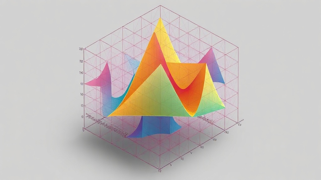
Consider a simple regression with two predictors, X1 and X2, and a response Y. The model tries to find coefficients $\beta_1$ and $\beta_2$ such that $Y \approx \beta_0 + \beta_1 X_1 + \beta_2 X_2$. If X1 and X2 are highly correlated, they are nearly collinear. Geometrically, this means the vectors representing X1 and X2 are almost parallel. The model's task is to project the vector Y onto the plane spanned by X1 and X2. When X1 and X2 are nearly parallel, the plane they span is very 'thin' or elongated. Small changes in the data, or in the direction of Y relative to this thin plane, can cause the projection point (which determines the coefficients) to shift dramatically along the line of collinearity.
Think of it like trying to balance a long, thin plank on a pivot. If you nudge it slightly, the ends can swing wildly. Similarly, in a highly multicollinear model, a small change in the data can lead to a large change in the estimated coefficients. This is because the model can 'satisfy' the regression equation by redistributing the explained variance between the correlated predictors. If X1 and X2 are perfectly collinear, the model cannot even begin to estimate unique coefficients for them; it can only estimate a combined effect. When they are 'nearly' collinear, the solution becomes numerically unstable, leading to the 'exploding' betas.
The Impact of Exploding Betas
When multicollinearity causes coefficients to fluctuate, several critical issues arise:
- Unreliable Coefficient Estimates: The magnitude and even the sign of the coefficients can change drastically with minor data alterations. A variable that appears statistically significant and positive in one model iteration might become insignificant or negative in another, making it impossible to trust the interpretation of individual variable effects.
- Inflated Standard Errors: The standard errors of the affected coefficients become very large. This means the confidence intervals around these coefficients widen considerably, making it difficult to conclude that any predictor variable has a statistically significant effect on the outcome, even if the overall model fit is good.
- Sensitivity to Model Specification: The model becomes highly sensitive to the inclusion or exclusion of other variables, or even small changes in the dataset. This fragility undermines the robustness and generalizability of the model.
- Misleading Significance Tests: While the overall F-statistic for the model might still be significant (indicating that the predictors, as a group, explain a significant portion of the variance), the individual t-tests for the correlated predictors will likely show non-significance due to the inflated standard errors.
Detecting and Mitigating Multicollinearity
Fortunately, multicollinearity is not an insurmountable problem. Several methods can help detect and mitigate it:
Detection Methods
- Variance Inflation Factor (VIF): This is the most common metric. VIF measures how much the variance of an estimated regression coefficient is increased because of collinearity. A VIF value above 5 or 10 (depending on the field's convention) is often considered indicative of problematic multicollinearity. VIF is calculated for each predictor variable.
- Correlation Matrix: Examining pairwise correlations between independent variables can reveal strong linear relationships. However, this only detects pairwise collinearity and misses more complex, multi-variable dependencies.
- Eigenvalues of the Correlation Matrix: A more sophisticated geometric approach involves analyzing the eigenvalues of the correlation matrix of the predictor variables. Small eigenvalues (or condition indices) suggest that the predictor variables are nearly linearly dependent.
Mitigation Strategies
- Remove Redundant Variables: If two variables are highly correlated and measure essentially the same underlying construct (e.g., height in inches and height in centimeters), remove one.
- Combine Variables: Create composite variables or indices by averaging or summing highly correlated predictors, provided this makes theoretical sense. Principal Component Analysis (PCA) can also be used to create uncorrelated components.
- Ridge Regression or Lasso: These are regularization techniques that add a penalty term to the regression objective function. Ridge regression (L2 regularization) shrinks coefficients and can handle multicollinearity by introducing a small amount of bias to reduce variance. Lasso (L1 regularization) can also perform variable selection by driving some coefficients exactly to zero.
- Gather More Data: Sometimes, multicollinearity is an artifact of a small or unrepresentative sample. A larger, more diverse dataset might naturally reduce the correlations between predictors.
- Centering Variables: For polynomial regression or models with interaction terms, centering the variables (subtracting their mean) before creating the interaction or polynomial terms can sometimes reduce multicollinearity.
Conclusion: A Geometric Perspective for Robust Models
Understanding multicollinearity through its geometric interpretation—the near-parallel alignment of predictor variable vectors in feature space—provides a deeper insight into why regression coefficients become unstable. This geometric perspective highlights that the problem is not just about correlation, but about the dimensionality and linear dependency within the predictor space. By employing detection methods like VIF and mitigation strategies such as regularization or variable selection, practitioners can build more robust and interpretable regression models, avoiding the pitfalls of 'exploding' betas and ensuring more reliable insights from their data.