
Introduction: The Gateway to Data Analysis
Embarking on a data science or machine learning project invariably begins with a crucial step: getting your data into a usable format within your chosen development environment. For many, this environment is a Jupyter Notebook, and the de facto standard for data manipulation in Python is the Pandas library. Loading a dataset, typically from a CSV file, is the foundational skill that unlocks all subsequent analysis, visualization, and modeling. This guide breaks down the process into clear, actionable steps, ensuring you can efficiently import your data and avoid common pitfalls.
Pandas provides a powerful and flexible DataFrame object, which is essentially a two-dimensional labeled data structure with columns of potentially different types. It's akin to a spreadsheet or a SQL table, but with far greater analytical capabilities. Understanding how to create and populate this DataFrame from external files is paramount.

Step 1: Importing the Pandas Library
Before you can leverage Pandas for data loading, you must first import the library into your Python script or Jupyter Notebook. The conventional practice is to import Pandas with the alias pd. This alias is universally recognized within the data science community, making your code more readable and interoperable with others' work.
The import statement is straightforward:
import pandas as pd
This command tells Python to find the Pandas library and make its functions and objects available under the shorthand name pd. Without this step, any attempt to use Pandas functions, such as read_csv, will result in a NameError.
Step 2: Loading Your Dataset with read_csv()
Once Pandas is imported, the next logical step is to load your dataset. For datasets stored in Comma Separated Values (CSV) format, Pandas offers the highly efficient read_csv() function. This function is the workhorse for CSV data ingestion.
The basic syntax for loading a CSV file looks like this:
df = pd.read_csv("your_dataset.csv")
Let's dissect this command:
pd: This is the alias for the Pandas library, as established in Step 1.read_csv(): This is the specific Pandas function designed to read data from a CSV file. It can handle various delimiters, encoding issues, and other CSV-specific complexities, although its default settings work for most standard CSVs."your_dataset.csv": This is the argument passed to theread_csv()function. It represents the path to your CSV file. If the CSV file is in the same directory as your Jupyter Notebook, you can simply use its filename. If it's in a different directory, you'll need to provide the full or relative path. For example,"data/raw/your_dataset.csv"or"/Users/yourname/Documents/datasets/your_dataset.csv".df: This is a variable name. By convention, datasets loaded into Pandas are stored in variables nameddf, which is short for DataFrame. This variable will hold the entire dataset as a Pandas DataFrame object, ready for manipulation.
When you execute this line, Pandas parses the CSV file, interprets the data, and constructs a DataFrame. The first row of the CSV is typically inferred as the header row containing column names, and subsequent rows are treated as data entries.
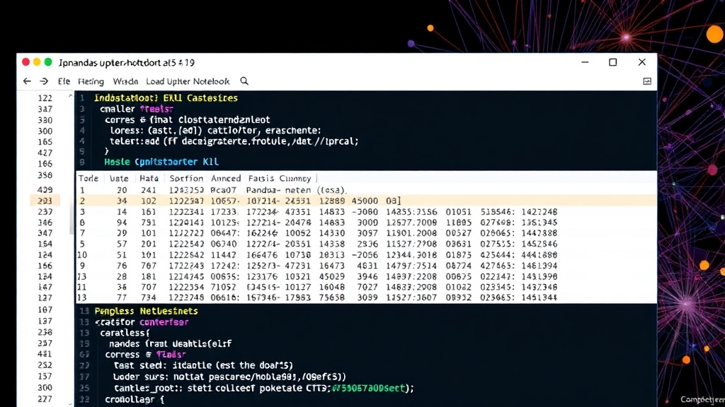
Understanding the Pandas DataFrame
The result of pd.read_csv() is a Pandas DataFrame. It's crucial to understand what this object is and how it's structured. A DataFrame is a tabular data structure, much like a table in a database or a sheet in Excel. It has rows and columns.
Key characteristics of a DataFrame include:
- Columns: Each column has a name (usually derived from the CSV header) and a data type (e.g., integer, float, string, boolean, datetime).
- Index: Rows are identified by an index, which is a sequence of labels. By default, Pandas assigns a numerical index starting from 0.
- Data: The cells within the DataFrame contain the actual data values from your dataset.
After loading, you can inspect your DataFrame to ensure it loaded correctly. Common first steps include:
df.head(): Displays the first 5 rows of the DataFrame.df.tail(): Displays the last 5 rows.df.info(): Provides a concise summary of the DataFrame, including the column names, non-null counts, and data types.df.describe(): Generates descriptive statistics for numerical columns (count, mean, std, min, max, quartiles).
These commands are essential for a quick validation of your data import.
Handling Different CSV Formats and Options
While pd.read_csv() is powerful, real-world data often requires more nuanced handling. CSV files don't always strictly adhere to the comma-separated standard.
Specifying Delimiters
Some files use semicolons, tabs, or other characters as separators instead of commas. You can specify the delimiter using the sep parameter:
df = pd.read_csv("data_with_semicolons.csv", sep=";")

df = pd.read_csv("data_with_tabs.tsv", sep="\t")
Handling Headers
If your CSV file does not have a header row, or if the header is on a different row, you can control this behavior:
header=None: Use this if your file has no header. Pandas will assign default numerical column names (0, 1, 2, ...).names=[...]: Provide a list of column names to assign to your DataFrame. This is often used in conjunction withheader=None.header=N: Specifies that the header is on the Nth row (0-indexed).
# No header in the CSV file, assign custom names
df = pd.read_csv("no_header_data.csv", header=None, names=["col1", "col2", "col3"])
Encoding Issues
Text files can be encoded in various ways (e.g., UTF-8, ISO-8859-1). If you encounter errors related to character encoding, you might need to specify the correct encoding:
df = pd.read_csv("data_with_utf16.csv", encoding="utf-16")
Common encodings to try if UTF-8 fails include 'latin1' or 'ISO-8859-1'.
Selecting Specific Columns
Sometimes, you might only need a subset of columns from a large dataset. Loading only necessary columns can save memory and processing time.
# Load only 'UserID' and 'PurchaseAmount' columns
df = pd.read_csv("sales_data.csv", usecols=["UserID", "PurchaseAmount"])
Parsing Dates
If your dataset contains date or timestamp columns, it's often beneficial to parse them directly into datetime objects during loading, rather than as strings.
# Parse 'OrderDate' and 'ShipDate' columns as dates
df = pd.read_csv("orders.csv", parse_dates=["OrderDate", "ShipDate"])
This allows for easier time-based analysis and manipulation.
Common Issues and Troubleshooting
While Pandas makes loading data straightforward, issues can arise:
- FileNotFoundError: The most common error. Ensure the file path is correct and the file exists at that location relative to your notebook. Check for typos in the filename.
- Empty DataFrame: If
df.head()returns nothing, the file might be empty, or the delimiter might be incorrect, leading Pandas to interpret the file structure improperly. - Incorrect Data Types: Numbers might be loaded as strings, or dates as objects. Use
df.info()to check types anddf.astype()orpd.to_numeric()/pd.to_datetime()for conversions after loading ifread_csvoptions don't suffice. - Memory Errors: For very large datasets, loading the entire file might exceed your system's RAM. Consider using
chunksizeto read the file in pieces, or use more memory-efficient data types.
Conclusion: Beyond the First Load
Successfully loading a dataset into your Jupyter Notebook using Pandas is a fundamental skill. The pd.read_csv() function, with its numerous parameters, offers robust capabilities to handle diverse data formats. By mastering these basics and understanding common troubleshooting techniques, you establish a solid foundation for all your subsequent data exploration and machine learning endeavors. The DataFrame is your canvas; now you're ready to start painting with data.