Part 1: Linear Regression — What the Model Actually Does
Linear regression is a cornerstone of predictive modeling in machine learning. Its core function is to discern the relationship between a set of input features and a continuous target variable. In its simplest form, it fits the best possible straight line through the data points. When dealing with multiple input features, this 'line' expands into a higher-dimensional construct known as a hyperplane, but the fundamental principle remains identical.
Mathematically, for multiple features, the linear regression model is expressed as:
ŷ = β₀ + β₁x₁ + β₂x₂ + ... + βₙxₙ
Here, ŷ represents the predicted value. β₀ is the intercept term, signifying the value of the target when all features are zero. β₁ through βₙ are the coefficients associated with each feature (x₁ through xₙ). These coefficients are crucial; they quantify the extent to which each input feature influences the prediction. A positive coefficient indicates that an increase in the feature's value leads to an increase in the predicted value, while a negative coefficient suggests the opposite.
How Coefficients Are Found: Ordinary Least Squares (OLS)
The process of determining the optimal coefficients (β values) for a linear regression model hinges on minimizing a specific error metric: the Residual Sum of Squares (RSS). The residuals are the differences between the actual observed values (yᵢ) and the values predicted by the model (ŷᵢ) for each data point i.
The RSS is calculated as:
RSS = Σ(yᵢ - ŷᵢ)²
The goal of Ordinary Least Squares (OLS) is to find the set of coefficients that yields the smallest possible RSS. This is achieved by calculating the partial derivatives of the RSS with respect to each coefficient and setting them to zero, then solving the resulting system of linear equations. Geometrically, OLS seeks to position the regression line (or hyperplane) such that the sum of the squared vertical distances from each data point to the line is minimized. This method is computationally efficient for smaller datasets but can become resource-intensive for very large ones.
Part 2: The Problem of Overfitting
While linear regression is powerful, it's not immune to a common machine learning pitfall: overfitting. Overfitting occurs when a model learns the training data too well, including its noise and random fluctuations. Such a model will perform exceptionally well on the data it was trained on but will generalize poorly to new, unseen data. This leads to high variance and unreliable predictions in real-world applications.
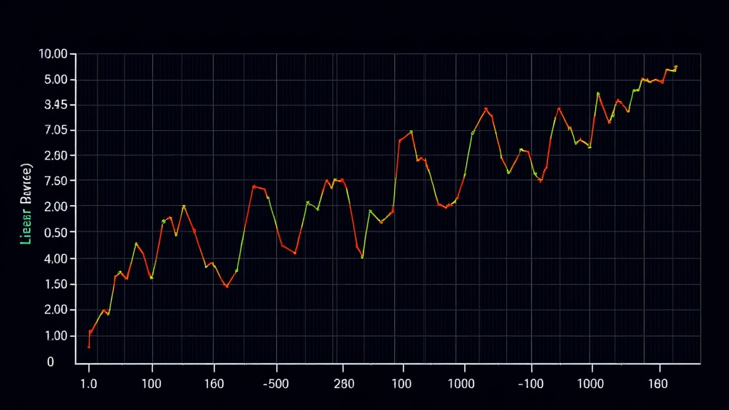
Consider a scenario with a very complex dataset that has many features, some of which might be irrelevant or redundant. A standard linear regression model, especially one with a high degree polynomial, could try to perfectly capture every single data point. This results in a highly convoluted decision boundary or regression line that wiggles excessively to accommodate outliers. While the error on the training set might approach zero, this intricate model fails to capture the underlying, simpler relationship that truly governs the data. It has essentially memorized the training examples rather than learned the general pattern.
Part 3: Regularization — Taming the Model
Regularization techniques are designed to combat overfitting by adding a penalty term to the model's loss function. This penalty discourages the model from assigning excessively large coefficients to features. By constraining the magnitude of the coefficients, regularization effectively simplifies the model, making it less sensitive to the noise in the training data and improving its ability to generalize to new data. Think of it like putting reins on a powerful horse; you're not stopping it from running, but you're ensuring it stays on a controlled path.
Ridge Regression (L2 Regularization)
Ridge regression introduces a penalty proportional to the square of the magnitude of the coefficients. The modified loss function becomes:
Loss = RSS + λ Σ(βⱼ)²
Here, λ (lambda) is the regularization parameter, a non-negative tuning parameter. It controls the strength of the penalty. A higher λ means a stronger penalty, leading to smaller coefficients. If λ = 0, Ridge regression is equivalent to ordinary least squares. As λ approaches infinity, the coefficients approach zero. Ridge regression shrinks the coefficients towards zero but does not typically force them to be exactly zero, meaning it retains all features in the model, albeit with reduced influence from those with larger coefficients.
Lasso Regression (L1 Regularization)
Lasso regression, on the other hand, uses a penalty proportional to the absolute value of the coefficients. Its loss function is:
Loss = RSS + λ Σ|βⱼ|
The key difference here is that the L1 penalty can force some coefficients to become exactly zero. This feature makes Lasso regression useful for feature selection. If a coefficient is driven to zero, it implies that the corresponding feature has little to no predictive power for the target variable, effectively removing it from the model. This can lead to sparser, more interpretable models, especially when dealing with a high-dimensional dataset where many features might be irrelevant.
Elastic Net Regression
Elastic Net regression combines both L1 and L2 penalties. It aims to leverage the strengths of both Ridge and Lasso. It includes both the squared magnitude penalty (from Ridge) and the absolute magnitude penalty (from Lasso) in its loss function. This approach can be beneficial when dealing with highly correlated features, as it tends to select groups of correlated variables together, unlike Lasso which might arbitrarily pick one and zero out others. The Elastic Net has two tuning parameters: λ (overall regularization strength) and α (the mixing parameter between L1 and L2 penalties).
Part 4: Choosing the Right Regularization Parameter (λ)
The performance of regularized models heavily depends on the choice of the regularization parameter, λ. An inappropriate λ can lead to underfitting (if λ is too high, shrinking coefficients too much) or overfitting (if λ is too low, not penalizing enough). The standard method for selecting the optimal λ is through cross-validation.
In k-fold cross-validation, the training data is split into 'k' equal-sized folds. The model is trained 'k' times. In each iteration, one fold is held out as the validation set, and the model is trained on the remaining k-1 folds. The performance is then evaluated on the held-out fold. This process is repeated for various values of λ. The λ that yields the best average performance across all k validation folds is selected as the optimal parameter. This empirical approach ensures that the chosen regularization strength balances model complexity and generalization ability.
Conclusion: Building Robust Models
Linear regression provides a fundamental tool for understanding relationships in data. However, its susceptibility to overfitting necessitates techniques like regularization. Ridge, Lasso, and Elastic Net regression offer powerful mechanisms to control model complexity by penalizing large coefficients, thereby improving generalization performance. By carefully tuning the regularization parameter through methods like cross-validation, data scientists can build more robust and reliable machine learning models capable of performing well on unseen data.