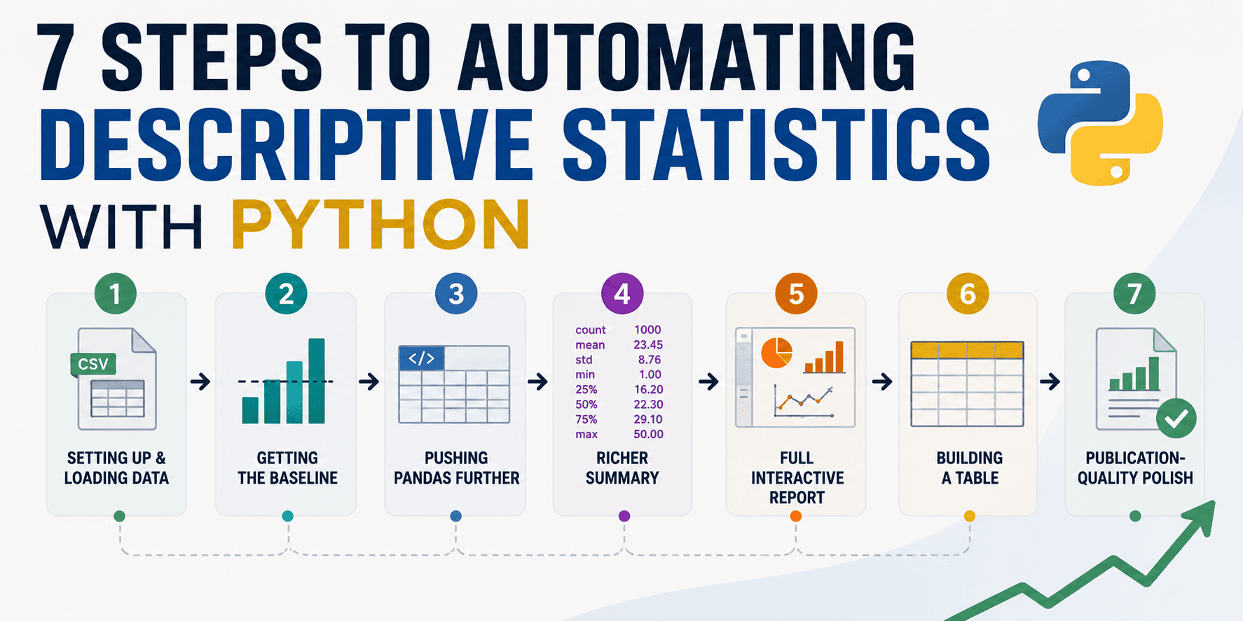
Automating Descriptive Statistics in Python
Manual calculation of descriptive statistics for every column in a dataset is a tedious and error-prone process. Developers and data professionals often find themselves repeatedly writing functions like mean(), std(), min(), and max() for each variable. This repetitive task not only consumes valuable time but also increases the likelihood of introducing errors, especially in large or complex datasets. Fortunately, Python's rich ecosystem of libraries offers elegant solutions to automate this process, enabling the generation of comprehensive, publication-ready summary tables with minimal effort.
Automating descriptive statistics is crucial for efficient data exploration and reporting. It allows for a quicker understanding of data distributions, central tendencies, and variability. This automation is particularly beneficial when dealing with datasets that are frequently updated or when performing iterative analysis. By setting up an automated workflow, you can ensure consistency and accuracy in your statistical summaries, freeing up cognitive resources to focus on deeper insights and modeling rather than routine calculations.
Step 1: Importing Necessary Libraries
The first step in automating descriptive statistics is to import the required Python libraries. The primary libraries for data manipulation and statistical analysis are pandas and numpy. pandas provides the DataFrame structure, which is ideal for handling tabular data, and offers built-in methods for statistical calculations. numpy, on the other hand, is fundamental for numerical operations and often works in conjunction with pandas.
For generating summary tables, especially those formatted for publication, additional libraries might be useful. However, for the core task of calculating statistics, pandas is usually sufficient. If you intend to export these tables to specific formats like LaTeX or Excel, libraries like tabulate or pandas' own to_latex() and to_excel() methods come into play.
import pandas as pd
import numpy as np
Step 2: Loading Your Dataset
Once the libraries are imported, the next step is to load your dataset into a pandas DataFrame. The method for loading will depend on the format of your data. Common formats include CSV, Excel, SQL databases, and JSON. Pandas provides convenient functions for each of these.
For instance, if your data is in a CSV file named data.csv, you would use pd.read_csv(). Similarly, pd.read_excel() is used for Excel files, and pd.read_sql() for data from SQL databases. It is essential to ensure that the data is loaded correctly, with appropriate data types assigned to each column, as this can impact the accuracy of subsequent statistical calculations.
# Example: Loading a CSV file
df = pd.read_csv('your_dataset.csv')

# Display the first few rows to verify loading
print(df.head())
Step 3: Calculating Basic Descriptive Statistics
Pandas DataFrames have a built-in method, .describe(), which is a powerful tool for generating a summary of central tendency, dispersion, and shape of a dataset’s distribution, excluding NaN values. By default, it computes count, mean, standard deviation, minimum, 25th percentile, median (50th percentile), 75th percentile, and maximum for numerical columns.
To get a more comprehensive set of descriptive statistics, you can pass arguments to the .describe() method. For example, to include the median, skewness, and kurtosis, you can use the include='all' parameter for all columns or specify a list of statistics you want to compute.
# Basic descriptive statistics for numerical columns
descriptive_stats = df.describe()
print(descriptive_stats)

# Including all columns (including non-numeric if possible, though often results in NaN for them)
# and specifying additional statistics
descriptive_stats_all = df.describe(include='all', percentiles=[.25, .5, .75, .9, .95, .99])
print(descriptive_stats_all)
Step 4: Customizing Statistics and Handling Data Types
The .describe() method is excellent, but sometimes you need specific statistics not included by default, or you need to handle categorical data differently. For numerical columns, you can manually calculate additional metrics like skewness, kurtosis, variance, or the number of unique values using pandas or numpy functions.
For categorical columns, .describe() with include='object' or include='category' provides count, unique values, top occurring value, and its frequency. You can extend this by calculating the mode, value counts for specific categories, or proportions.
A robust automation script should also handle missing values (NaN). You can choose to fill them, drop them, or report their count and percentage separately. The decision depends on the analysis context. For instance, calculating the percentage of missing values per column is a common and useful statistic.
# Calculating additional statistics for numerical columns
variance = df.var()
skewness = df.skew()
kurtosis = df.kurt()

# Calculating statistics for categorical columns
categorical_stats = df.describe(include=['object', 'category'])

# Calculating missing value counts and percentages
missing_counts = df.isnull().sum()
missing_percentages = (missing_counts / len(df)) * 100

# Combining these into a custom summary
custom_summary = pd.DataFrame({
    'count': df.count(),
    'mean': df.mean(numeric_only=True),
    'std': df.std(numeric_only=True),
    'min': df.min(numeric_only=True),
    '25%': df.quantile(0.25, numeric_only=True),
    '50%': df.quantile(0.5, numeric_only=True),
    '75%': df.quantile(0.75, numeric_only=True),
    'max': df.max(numeric_only=True),
    'variance': variance,
    'skewness': skewness,
    'kurtosis': kurtosis,
    'missing_count': missing_counts,
    'missing_percentage': missing_percentages
})

# For object/category columns, you might want to add:
# 'unique': df.nunique(),
# 'top': df.mode().iloc[0] # This gets the first mode if multiple exist

print(custom_summary)
Step 5: Structuring the Output Table
The raw output from pandas methods is functional but may not be immediately publication-ready. The goal is to create a clean, informative table. This often involves reshaping the DataFrame, renaming columns, and formatting the numerical values.
You might want to transpose the table so that statistics are rows and variables are columns, or vice-versa, depending on the desired presentation. Formatting numbers to a consistent number of decimal places is crucial for readability and professional appearance. Pandas' .round() method is perfect for this. For more advanced formatting, such as creating LaTeX tables, pandas offers methods like .to_latex(), which can handle many presentation aspects automatically.
Consider creating a function that takes a DataFrame and returns a formatted summary DataFrame. This function can encapsulate all the steps from calculation to formatting, making the automation truly repeatable.
def create_summary_table(dataframe):
    # Calculate core statistics
    summary = dataframe.describe(include='all', percentiles=[.25, .5, .75]).transpose()

    # Add custom statistics if needed (e.g., variance, skew, kurtosis)
    # Example: Adding variance
    summary['variance'] = dataframe.var(numeric_only=True)

    # Handle missing values
    summary['missing_count'] = dataframe.isnull().sum()
    summary['missing_percentage'] = (summary['missing_count'] / len(dataframe)) * 100

    # Format numerical columns
    # Select columns that are numeric in the summary DataFrame for formatting
    numeric_cols_in_summary = summary.select_dtypes(include=np.number).columns
    summary[numeric_cols_in_summary] = summary[numeric_cols_in_summary].round(3)

    # Rename columns for clarity if needed
    summary = summary.rename(columns={'50%': 'median'})

    return summary

publication_ready_table = create_summary_table(df)
print(publication_ready_table)
Step 6: Exporting the Summary Table
Once the summary table is structured and formatted, the final step is to export it. Common export formats include CSV, Excel, and LaTeX. Pandas makes this straightforward with methods like .to_csv(), .to_excel(), and .to_latex().
Saving to CSV is ideal for general data exchange. Saving to Excel is useful for sharing with stakeholders who primarily use spreadsheet software. For academic papers or reports that require precise formatting, exporting to LaTeX is invaluable, as it integrates seamlessly into LaTeX documents, preserving tables' structure and appearance.
When exporting, pay attention to options like including the index, specifying file paths, and handling potential encoding issues. For LaTeX, consider options for multi-page tables or specific environments.
# Export to CSV
publication_ready_table.to_csv('descriptive_stats_summary.csv')

# Export to Excel
publication_ready_table.to_excel('descriptive_stats_summary.xlsx')

# Export to LaTeX
try:
    publication_ready_table.to_latex('descriptive_stats_summary.tex', index=True)
except ImportError:
    print("Note: 'tabulate' library might be needed for to_latex(). Install it with: pip install tabulate")
Step 7: Scheduling and Integrating into Workflows
The ultimate goal of automation is to integrate these processes into regular workflows. This could mean scheduling the script to run automatically when new data arrives, or triggering it as part of a larger data processing pipeline. Tools like Apache Airflow, Luigi, or even simple cron jobs can be used to schedule Python scripts.
For data scientists and analysts, this means that as soon as new data is available, a comprehensive statistical summary is generated, providing immediate insights. This allows for a more agile approach to data analysis and reporting, ensuring that decisions are based on the most current information. The automation removes the human bottleneck, making the data analysis cycle significantly faster and more reliable.
Consider creating a Python package or module for your custom summary generation function. This promotes reusability across different projects and teams, standardizing how descriptive statistics are reported within an organization. Version control for these scripts and functions is also critical to track changes and ensure reproducibility.