The Challenge: Computational Load in AI
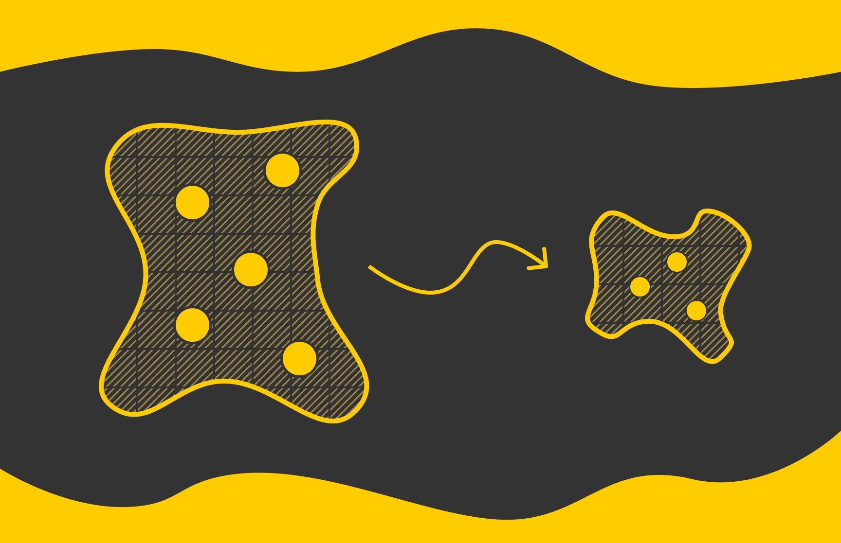
Modern machine learning, particularly generative AI applied to complex data like text and images, faces a significant hurdle: heavy computation. Processing and generating this unstructured data demands immense resources. To combat this, a core strategy involves compressing input data into a more manageable, lower-dimensional representation while crucially retaining the essential information. This is where autoencoders shine.
What is an Autoencoder?
An autoencoder is a type of artificial neural network designed for unsupervised learning, primarily used for dimensionality reduction and feature learning. It learns a compressed representation of the input data, known as the latent space, in an efficient manner. The network consists of two main parts: an encoder and a decoder.
The Encoder: Compressing Information
The encoder's job is to take the input data and transform it into a lower-dimensional representation. It maps the input, which could be a high-dimensional vector (like the pixels of an image), to a compressed representation in the latent space. This compression is achieved through a series of layers that progressively reduce the dimensionality of the data. The encoder learns to identify and retain the most salient features of the input, discarding redundant or less important information.
The Latent Space: The Compressed Core
The latent space is the bottleneck of the autoencoder. It's a lower-dimensional representation of the input data, capturing its most important characteristics. Think of it less like a database and more like a highly distilled summary of the original information. If the original data is a detailed photograph, the latent space representation is like a sketch that captures the essence of the subject – its key shapes and forms, but not every minute detail. The dimensionality of the latent space is a hyperparameter that can be tuned; a smaller dimension implies greater compression.
The Decoder: Reconstructing the Data
The decoder's role is the inverse of the encoder. It takes the compressed representation from the latent space and attempts to reconstruct the original input data as accurately as possible. It learns to map the latent representation back to the original high-dimensional space. The goal is for the reconstructed output to be as close as possible to the original input.
Training an Autoencoder: The Reconstruction Loss
Autoencoders are trained by minimizing a loss function that measures the difference between the original input and the reconstructed output. This is often called the reconstruction loss. Common loss functions include Mean Squared Error (MSE) for continuous data or Binary Cross-Entropy for binary data. During training, the network adjusts its weights to minimize this loss, effectively learning to encode the data into the latent space and then decode it back with minimal information loss.
Types of Autoencoders
While the basic autoencoder is foundational, several variations exist, each tailored for specific tasks:
Denoising Autoencoders
These are trained to reconstruct a clean input from a corrupted version. The input data is intentionally corrupted (e.g., by adding random noise or masking parts of it), and the autoencoder learns to remove the noise, thus learning more robust features. This is akin to a skilled restorer carefully repairing a damaged painting, focusing on bringing out the original detail while ignoring the damage.
Variational Autoencoders (VAEs)
VAEs are a more sophisticated type that learns a probability distribution for the latent space. Instead of mapping an input to a single point, it maps it to a distribution (typically a Gaussian). This probabilistic approach allows VAEs to generate new data samples by sampling from the learned latent distribution and decoding them. This is crucial for generative modeling, enabling the creation of novel images, text, or other data that resemble the training data but are not direct copies.
Sparse Autoencoders
These impose sparsity constraints on the latent representation. This means that only a small number of neurons in the latent layer should be active for any given input. This encourages the network to learn more meaningful and disentangled features.
Applications of Autoencoders
Autoencoders have a wide range of practical applications:
- Dimensionality Reduction: Compressing high-dimensional data into a lower-dimensional space for visualization, efficient storage, or faster processing in subsequent ML tasks.
- Feature Learning: Extracting meaningful features from raw data, which can then be used for classification or clustering.
- Anomaly Detection: Autoencoders trained on normal data will have a high reconstruction error when presented with anomalous data, as they struggle to reconstruct patterns they haven't seen.
- Generative Modeling: As seen with VAEs, they can be used to generate new data samples.
- Image Denoising and Inpainting: Removing noise from images or filling in missing parts.
The Significance of Latent Space
The latent space is the heart of an autoencoder's power. It represents a compressed, abstract version of the input data. By learning this representation, autoencoders achieve several key benefits:
- Reduced Computational Cost: Working with lower-dimensional data significantly reduces the computational resources needed for further analysis or generation.
- Noise Reduction: The compression process often filters out noise, leading to cleaner data representations.
- Feature Extraction: The latent space can reveal underlying structures and relationships in the data that are not apparent in the raw, high-dimensional form.
Understanding autoencoders and their latent space is fundamental for anyone working with large datasets and complex AI models, offering a pathway to more efficient and effective machine learning.