The Problem: Visuals Masking Model Chaos
A Power BI dashboard can present a polished facade, but beneath the surface, the underlying data model might be a complete mess. The user sees the visuals, but their accuracy, flexibility, and the ability to answer complex analytical questions hinge entirely on how the data is structured before reporting begins. Imagine analyzing Premier League match data to answer questions like: Which teams perform better at home? Which teams struggle away? Do match statistics change during different periods of the season? Are there patterns in fouls, cards, or referee decisions? While these questions can be answered with compelling visuals, the foundational question that must be addressed first is: How should the data be structured so that the same model can support diverse reports and analytical questions? This is the essence of data modelling in Power BI.
What is Data Modelling in Power BI?
Data modelling in Power BI is the process of organizing your data into tables and, critically, defining the relationships between these tables. A well-structured model is not just about aesthetics; it directly impacts the ease of building reports, managing filters, writing complex DAX (Data Analytics Expressions) calculations, and maintaining excellent performance, especially as your data volume grows and changes. It’s about creating a logical framework that makes your data understandable and actionable.
Fundamental Modelling Approaches
There are several ways to structure your data, each with its own strengths and weaknesses. For the purposes of this discussion, we will explore three primary approaches: the flat table, the star schema, and the snowflake schema. We'll use a sample dataset, referred to as NovaMart, which contains detailed information about customers and their orders, to illustrate these concepts.
Approach 1: The Flat Table
A flat table, sometimes referred to as a denormalized table, consolidates transactional and descriptive data into a single, wide table. This approach is straightforward to set up and can be highly effective for smaller datasets where performance is not a significant concern. For instance, a raw sales table might contain all order details, customer information, and product specifics within its columns. However, as the dataset expands, managing and maintaining a single, massive table can become increasingly difficult. Redundancy is common, leading to larger file sizes and potential inconsistencies if updates are not applied uniformly across all records. While simple, it often sacrifices efficiency and scalability for ease of initial setup.

Approach 2: The Star Schema
The star schema is a widely adopted and highly recommended data modelling approach in Power BI and other business intelligence platforms. It organizes data into a central 'fact' table surrounded by several 'dimension' tables, resembling a star. The fact table contains the quantitative measurements or metrics of a business process (e.g., sales amount, quantity sold, profit). Dimension tables, on the other hand, contain descriptive attributes that provide context to the facts (e.g., customer details, product information, dates, locations).
The fact table typically has a composite primary key made up of foreign keys linking to each dimension table. Dimension tables usually have a single, unique primary key. This structure significantly reduces data redundancy. For example, instead of repeating customer address details for every sale a customer makes, the customer's information is stored once in the 'Customer' dimension table and linked via a customer ID. This design optimizes query performance and simplifies report creation because users can easily slice and dice measures by various dimensions. Power BI's engine is optimized to work efficiently with this structure, making DAX calculations faster and more manageable.
Approach 3: The Snowflake Schema
The snowflake schema is an extension of the star schema. In a snowflake schema, the dimension tables are further normalized. This means that a dimension table might be broken down into additional, smaller tables. For instance, a 'Product' dimension table in a star schema might include product category and sub-category names directly. In a snowflake schema, the 'Product' dimension might link to a separate 'Category' dimension table, which in turn links to a 'Department' dimension table.
The primary advantage of this normalization is further reduction in data redundancy and a potential saving in storage space. It enforces data integrity more strictly, as changes to a category name, for example, only need to be made in one place. However, this increased normalization comes at a cost: it creates more complex relationships between tables. Queries that need to traverse multiple levels of these normalized dimensions can become slower and more intricate to write and understand. For Power BI, where performance is key and the engine is already highly optimized for star schemas, the added complexity of a snowflake schema often outweighs its storage benefits, making the star schema generally the preferred choice.
Relationships in Power BI
Defining relationships between tables is the cornerstone of data modelling in Power BI. Power BI uses these relationships to connect data from different tables, allowing you to analyze them together. When you import data, Power BI attempts to auto-detect relationships based on column names and data types. However, you should always review and, if necessary, manually create or modify these relationships to ensure they are correct.
There are two main types of relationships:
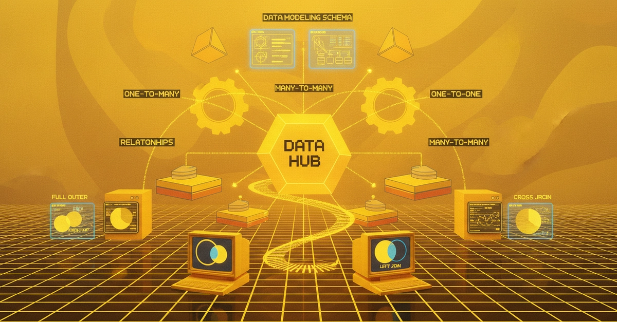
- One-to-Many: This is the most common type. A row in one table corresponds to many rows in another. For example, one customer can have many orders. The 'one' side is typically a dimension table (e.g., Customers), and the 'many' side is the fact table (e.g., Sales).
- One-to-One: Less common, where a row in one table corresponds to exactly one row in another. This might occur when splitting a very wide table into two for organizational or performance reasons.
- Many-to-Many: While possible, these are generally discouraged in Power BI data models as they can lead to ambiguity and performance issues. They often indicate a need to restructure the model, perhaps by introducing a bridging table.
The cross-filter direction is also a critical aspect of relationships. By default, filters flow from the 'one' side to the 'many' side (single direction). In some advanced scenarios, you might need a bi-directional cross-filter, but this should be used with caution as it can create ambiguity and performance bottlenecks.
Power Query Joins vs. Model Relationships
It's crucial to distinguish between joins performed in Power Query (during the data transformation stage) and relationships defined in the Power BI data model.
- Power Query Joins (Merge Queries): These are performed before the data is loaded into the Power BI model. You can perform various types of joins (Inner, Left Outer, Right Outer, Full Outer, Left Anti, Right Anti) to combine data from different tables into a single table. This is often used to create the fact and dimension tables that will populate your model. For example, you might join a sales transaction table with a product lookup table to bring product details directly into the sales table, effectively creating a flatter structure within Power Query before loading.
- Model Relationships: These are defined after the data is loaded into the Power BI model. They connect separate tables, allowing Power BI to interpret how data across these tables relates for reporting and analysis. This is the mechanism that enables slicing sales by product category, for instance, without having to duplicate all product information in the sales table.
Understanding this distinction is vital. Joins in Power Query create the structure of your tables, while relationships in the model enable analysis across those structures. For optimal performance and maintainability, it's generally recommended to perform necessary joins in Power Query to create well-defined fact and dimension tables, and then establish relationships between these tables within the Power BI model.
Why Good Data Modelling Matters
A poorly modelled dataset can lead to inaccurate reports, slow performance, and an inability to answer evolving business questions. It’s like building a house on a shaky foundation; no matter how beautiful the facade, the structure is compromised. Conversely, a robust, well-designed star schema allows for intuitive report building, efficient DAX calculations, and reliable insights. It empowers users to explore data confidently and provides a scalable platform for future reporting needs. If you're building reports in Power BI, investing time in understanding and implementing effective data modelling practices, particularly the star schema, is paramount to success.