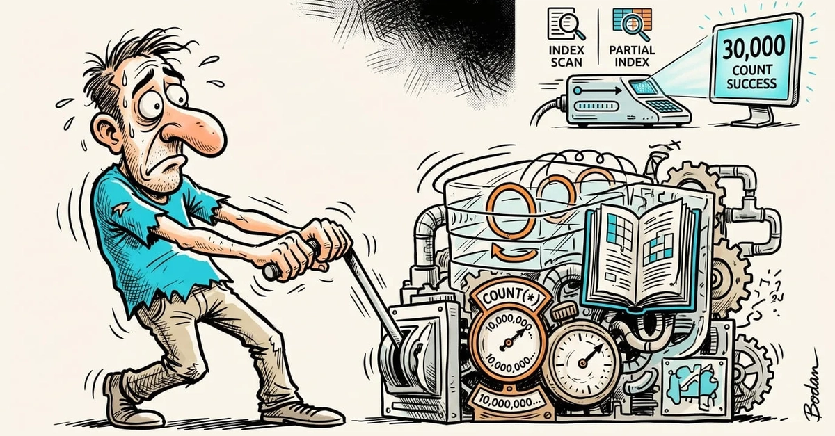
The Illusion of Simplicity in COUNT(*)
At first glance, a query like SELECT COUNT(*) FROM orders; appears deceptively simple. It asks for a single number, a summary statistic. Many developers assume that databases, especially mature ones like PostgreSQL, maintain an internal counter that can be read in constant time. This intuition, however, is incorrect. PostgreSQL does not keep a continuously updated, exact count of rows for every table. Instead, when an exact count is requested, the database must perform work to determine precisely how many rows are visible and relevant to the query at that moment.
This process becomes computationally expensive on large tables. PostgreSQL must scan the table or a relevant index to identify and count each visible row. The time taken for this operation is directly proportional to the number of rows that need to be examined, making it a significant bottleneck for applications that frequently query row counts on substantial datasets. The common misconception is that adding an index to the table will automatically accelerate this operation. While indexes are invaluable for speeding up data retrieval based on specific conditions (like WHERE column = value), they do not inherently solve the problem of calculating an exact total count efficiently.
How PostgreSQL Actually Counts Rows
When you execute COUNT(*), PostgreSQL's query planner evaluates the most efficient way to satisfy the request. For an exact count, it generally has two primary strategies:
- Full Table Scan: The database reads every single row in the table, increments a counter for each one, and returns the final value. This is often the most straightforward approach for small tables or when no suitable index exists.
- Index Scan: If a suitable index exists, PostgreSQL might scan the index instead of the table. An index contains entries for each row in the table, ordered by the indexed column(s). Scanning an index can be faster than scanning the table if the index is significantly smaller than the table itself (e.g., an index on a single integer column). However, even an index scan requires visiting a large number of index entries to count all visible rows.
The crucial point is that PostgreSQL needs to *examine* the rows (or index entries) to determine their visibility. Row visibility is managed through PostgreSQL's Multi-Version Concurrency Control (MVCC) system. Each row has associated transaction information that indicates whether it is visible to the current transaction. Therefore, a COUNT(*) operation isn't just reading a pre-computed value; it's actively determining the state of the data.
Consider an analogy: Imagine you have a massive library with millions of books. If someone asks for the exact number of books in the library, you can't just look at a sign that says "Total Books: X." You have to walk through every aisle, every shelf, and count each book. If some books are temporarily checked out or in repair (analogous to deleted or uncommitted rows), you need to verify their presence before counting. An index might be like a catalog of books by title, but to get the total count, you still need to go through the catalog and confirm each book's existence, which is still a significant undertaking.
Why Indexes Fall Short for COUNT(*)
The common instinct is to add an index on a column, or even a dummy column, hoping it will provide a shortcut for COUNT(*). However, this strategy is often ineffective for two main reasons:
- Index Structure: While an index contains an entry for each row, it's still a data structure that needs to be traversed. For a B-tree index, which is standard in PostgreSQL, `COUNT(*)` would involve traversing a significant portion of the leaf nodes to count all entries. This is often comparable in cost to a full table scan, especially if the index is wide or the table is very large.
- MVCC Complexity: Even if an index is scanned, PostgreSQL still needs to consult the row's TOAST pointers or tuple headers to determine visibility. This check adds overhead to each index entry examined, negating much of the potential performance gain. An index might help if it's a covering index that includes all columns needed for visibility checks, but this is rare and complex to maintain.
The query planner might choose an index scan if it estimates that the index is smaller than the table and scanning it will be faster. However, this is an estimation, and for very large tables, the cost of traversing a large index can still be substantial. Furthermore, if your COUNT(*) is part of a query with a WHERE clause, an index can be highly beneficial. But for a plain COUNT(*) on the entire table, its utility diminishes significantly.
Alternative Strategies for Faster Counts
Since traditional indexing is not a silver bullet for slow COUNT(*), developers and DBAs often turn to alternative methods:
- Approximate Counts: If an exact count is not strictly necessary, PostgreSQL offers functions like
reltuplesfrom thepg_classsystem catalog.SELECT reltuples::bigint FROM pg_class WHERE relname = 'orders';provides an estimate based on the lastANALYZEorVACUUMoperation. This is extremely fast but can be inaccurate, especially on tables with frequent inserts and deletes. The accuracy depends on how recently statistics were updated. - Materialized Views: For frequently needed exact counts, a materialized view can be created. This view would periodically run the
COUNT(*)query and store the result. Querying the materialized view is then very fast. However, the materialized view needs to be refreshed regularly to maintain accuracy, which itself can be a resource-intensive operation. - Triggers and Counters: A more complex approach involves using database triggers on insert and delete operations to maintain a separate counter table. Each time a row is inserted, the counter is incremented; each time a row is deleted, it's decremented. This provides an exact count in constant time (reading from the counter table) but adds overhead to every write operation and requires careful implementation to avoid race conditions and ensure consistency.
- Partitioning: For extremely large tables, partitioning can help. If you partition by a date range, for instance, you could get the count for a specific partition quickly. However, getting the total count across all partitions still requires summing counts from each partition, which might not be significantly faster than a full scan unless specific optimizations are in place or only a subset of partitions is queried.
The choice of strategy depends heavily on the specific application requirements: how frequently the count is needed, the acceptable level of inaccuracy, and the tolerance for additional complexity or write overhead.
The Unanswered Question: When is an Estimate Good Enough?
What often goes unaddressed is the threshold at which an approximate count becomes practically sufficient for most applications. Many dashboards, reporting tools, and user interfaces display row counts as an indicator of data volume or status. While developers may instinctively reach for an exact count, the reality is that a slightly stale or estimated number might be perfectly adequate for user perception and decision-making. The performance cost of guaranteeing absolute precision for COUNT(*) on massive tables is often disproportionately high compared to the actual business value derived from that precision at any given moment.
Ultimately, understanding that COUNT(*) is not a trivial operation and that indexes don't magically fix its performance is the first step. The next is to evaluate whether an exact count is truly a necessity or if a faster, albeit approximate, method will suffice for the given use case.