Gradient Descent: A Deep Dive into Optimization Algorithms

The Foundation of Optimization: Understanding Gradient Descent

Gradient Descent is a cornerstone algorithm in the field of machine learning and artificial intelligence, serving as a primary method for unconstrained mathematical optimization. At its heart, it's a first-order iterative algorithm designed to find the minimum of a differentiable multivariate function. The fundamental principle involves taking successive steps in the direction opposite to the gradient of the function at the current point. This methodical approach guides the algorithm along a path that progressively reduces the objective function, commonly referred to as the cost or loss function in machine learning contexts.

Think of Gradient Descent like a hiker trying to find the lowest point in a valley while blindfolded. The hiker can feel the slope of the ground beneath their feet (the gradient). To get to the bottom, they take steps in the direction that feels steepest downhill. They repeat this process, taking small steps, until they can no longer feel any downward slope, indicating they've reached a minimum.

This iterative process is crucial for training machine learning models, particularly neural networks. By minimizing the loss function, Gradient Descent helps the model learn the optimal parameters (weights and biases) that best fit the training data. While the basic concept is straightforward, its efficacy and speed can be significantly influenced by the choice of specific optimization algorithms and their hyperparameter settings, such as the learning rate.

Key Components of Gradient Descent

To understand Gradient Descent, it's essential to grasp its core components:

• Objective Function (Loss Function): This is the function we aim to minimize. In machine learning, it quantifies the error between the model's predictions and the actual target values. Common examples include Mean Squared Error (MSE) for regression and Cross-Entropy Loss for classification.
• Gradient: The gradient is a vector of partial derivatives of the objective function with respect to each of its parameters. It points in the direction of the steepest ascent of the function. For minimization, we move in the opposite direction of the gradient.
• Learning Rate (α): This hyperparameter controls the size of the steps taken during each iteration. A small learning rate can lead to slow convergence, while a large learning rate might cause the algorithm to overshoot the minimum or even diverge.
• Parameters (Weights and Biases): These are the variables of the objective function that the algorithm seeks to optimize. In neural networks, these are the weights and biases that define the network's structure and behavior.

The Basic Gradient Descent Algorithm (Batch Gradient Descent)

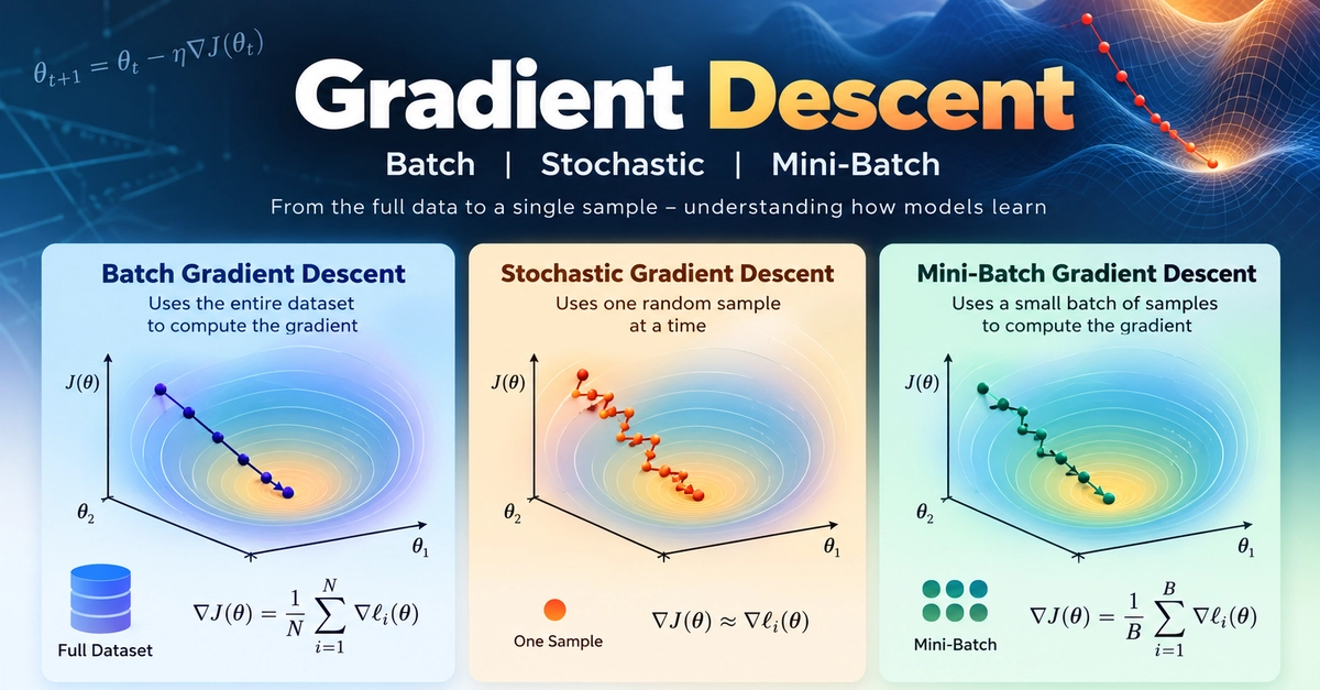
The most fundamental form of Gradient Descent is often referred to as Batch Gradient Descent. In this approach, the algorithm computes the gradient of the cost function using the entire training dataset in each iteration. This means that every single data point is used to calculate the gradient before updating the model's parameters.

The update rule for Batch Gradient Descent is:

θ = θ - α * ∇J(θ)

Where:

• θ represents the model parameters (weights and biases).
• α is the learning rate.
• ∇J(θ) is the gradient of the cost function J(θ) with respect to the parameters θ, computed using the entire dataset.

While Batch Gradient Descent guarantees convergence to the global minimum for convex cost functions and a local minimum for non-convex functions, it has significant drawbacks. Its primary limitation is computational inefficiency, especially for very large datasets. Calculating the gradient over the entire dataset can be extremely time-consuming and memory-intensive, making it impractical for many real-world applications.

Stochastic Gradient Descent (SGD)

To address the computational burden of Batch Gradient Descent, Stochastic Gradient Descent (SGD) was developed. Instead of using the entire dataset, SGD updates the model parameters using the gradient computed from a single, randomly selected training example at each iteration.

The update rule for SGD is:

θ = θ - α * ∇J(θ; x^(i); y^(i))

Where ∇J(θ; x^(i); y^(i)) is the gradient computed using only the i-th training example (x^(i), y^(i)).

The advantage of SGD is its speed. By performing updates more frequently (once per example rather than once per epoch), it can converge much faster, especially in the early stages of training. However, SGD's updates are much noisier due to the use of single data points. This noise can help it escape shallow local minima, but it also means the cost function fluctuates significantly, and the algorithm might not converge to the exact minimum but rather oscillate around it. To mitigate this, the learning rate is often gradually decreased over time (learning rate decay).

Mini-Batch Gradient Descent

Mini-Batch Gradient Descent offers a compromise between Batch Gradient Descent and Stochastic Gradient Descent. Instead of using the entire dataset or just a single data point, it uses a small, random subset of the training data, called a mini-batch, to compute the gradient in each iteration. Typical mini-batch sizes range from 32 to 256 examples.

The update rule for Mini-Batch Gradient Descent is:

θ = θ - α * ∇J(θ; x^(i:i+m); y^(i:i+m))

Where ∇J(θ; x^(i:i+m); y^(i:i+m)) is the gradient computed using a mini-batch of m examples.

This approach combines the benefits of both Batch and Stochastic Gradient Descent. It reduces the noise in parameter updates compared to SGD, leading to more stable convergence. It also offers significant computational advantages over Batch Gradient Descent, as it processes smaller batches of data. This makes Mini-Batch Gradient Descent the most commonly used variant in practice, striking a balance between convergence speed and stability, and allowing for efficient utilization of vectorized operations on modern hardware.

Beyond Basic Descent: Momentum and Adaptive Methods

While Batch, Stochastic, and Mini-Batch Gradient Descent are foundational, they can still face challenges, such as slow convergence in areas with small gradients or oscillations in steep ravines. To overcome these limitations, more advanced optimization algorithms have been developed. These often incorporate concepts like momentum or adapt the learning rate dynamically.

Momentum

Momentum is an optimization technique that helps accelerate Gradient Descent in the relevant direction and dampens oscillations. It introduces a 'velocity' term that accumulates past gradients. Imagine a ball rolling down a hill; it gains momentum and continues to roll even if it encounters a slight incline. In Gradient Descent, momentum helps the optimizer to continue moving in a consistent direction, smoothing out erratic updates caused by noisy gradients and speeding up convergence through flat regions.

Adaptive Learning Rate Methods

These methods adjust the learning rate for each parameter individually. They are particularly useful when dealing with sparse data or when different parameters have vastly different scales. Some popular adaptive methods include:

• AdaGrad (Adaptive Gradient): Adapts the learning rate based on the historical sum of squared gradients for each parameter. It decreases the learning rate for parameters that have received frequent updates and increases it for parameters with infrequent updates. However, it can cause the learning rate to decay too aggressively and stop learning prematurely.
• RMSprop (Root Mean Square Propagation): Addresses AdaGrad's diminishing learning rate by using an exponentially decaying average of squared gradients instead of the sum. This helps to prevent the learning rate from shrinking too quickly.
• Adam (Adaptive Moment Estimation): Combines the ideas of momentum and RMSprop. It computes adaptive learning rates for each parameter using estimates of both the first moment (mean) and the second moment (uncentered variance) of the gradients. Adam is widely regarded as one of the most effective and robust optimization algorithms for deep learning.

These advanced methods, by incorporating momentum or adaptive learning rates, allow neural networks to train more efficiently and effectively, especially in complex and high-dimensional spaces. The choice of optimizer can significantly impact the final performance of a machine learning model.