The Peril of Peeking: Why Early Wins Deceive
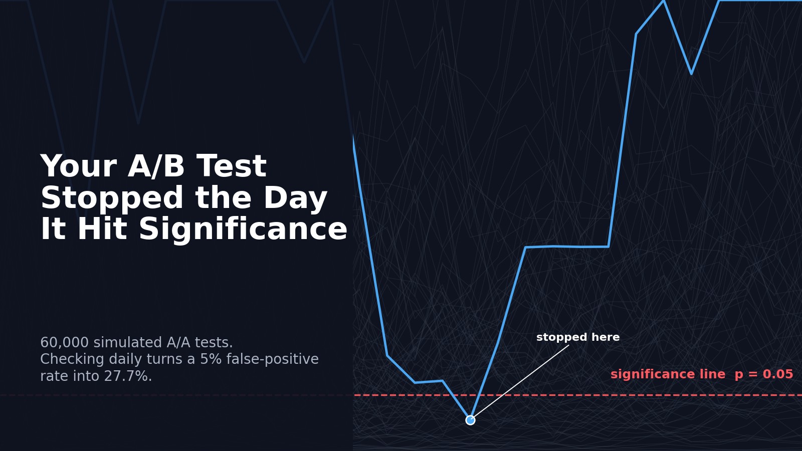
In the fast-paced world of product development and data science, the temptation to declare victory early in an A/B test is immense. A key metric crosses the seemingly sacred p < 0.05 significance level, and the impulse is to stop, analyze, and implement. This practice, however, is a statistical siren song, luring teams towards flawed decisions. Checking an A/B test until it crosses p < 0.05 can turn a nominal 5 percent false-positive rate into almost 28 percent. This is not a minor statistical anomaly; it's a fundamental distortion of probability that can lead to deploying changes that offer no real benefit, or worse, actively harm user experience.
Consider the standard A/B testing framework. We set a null hypothesis (e.g., variant B has no effect on conversion rate compared to variant A) and an alternative hypothesis (variant B has a positive effect). We collect data and calculate a p-value, which represents the probability of observing the data, or more extreme data, if the null hypothesis were true. If this p-value is below our chosen significance level (alpha, typically 0.05), we reject the null hypothesis and conclude there is a statistically significant difference. This 5% alpha is intended to mean that, if we ran the experiment many times and the null hypothesis was always true, we would incorrectly reject it only 5% of the time.
The problem arises when we don't pre-specify the duration or sample size of the test. Instead, we continuously monitor the results. Each time we check, we are essentially performing a new, albeit related, hypothesis test. This sequential testing, or "peeking," inflates the overall probability of a Type I error – a false positive. Imagine flipping a coin. If you decide to stop as soon as you see heads, you'll get heads very quickly. But if you decide to flip it 100 times and stop at the first heads, you're much more likely to stop early. The more often you peek, the higher your chance of seeing something that looks significant purely by chance, even if the underlying truth is no difference.
Quantifying the Damage: A Simulation Study
To illustrate the severity of this issue, a seeded simulation can reveal the true extent of the damage. By simulating thousands of A/B tests where the null hypothesis is true (i.e., no real difference between variants), we can observe how often a false positive emerges when using an early stopping rule. The results are stark: stopping at the first instance of p < 0.05 can indeed push the actual false-positive rate towards 28%, or even higher, depending on the frequency of checks and the total number of observations.
Let's break down what this means in practice. If you run 100 A/B tests where no change actually improves performance, and you use a naive early stopping strategy, you might expect to incorrectly conclude that nearly 28 of those tests showed a win. Deploying changes based on these false positives means allocating engineering resources, potentially disrupting user flows, and wasting valuable time on initiatives that yield no genuine uplift. This is akin to a doctor prescribing a treatment based on a lab result that was a false positive – the consequences can be detrimental.
This phenomenon is not new; it's a well-documented issue in statistical process control and sequential analysis. However, its pervasive application in everyday A/B testing, often driven by a desire for rapid iteration, poses a significant threat to data-informed decision-making. The allure of a quick win blinds teams to the underlying statistical inflation.
Towards Honest Early Stopping: Valid Fixes
Fortunately, statistical methodologies exist to keep early stopping honest. These approaches adjust the significance threshold dynamically as more data is collected, ensuring the overall Type I error rate remains at the desired level (e.g., 5%).
One primary approach is using group sequential methods. These methods pre-define specific points at which the test can be stopped for efficacy or futility. At each interim analysis, the p-value threshold is adjusted. For example, if you plan to check at 25%, 50%, 75%, and 100% of the planned sample size, the p-value required to declare significance at the 25% mark will be much lower than 0.05, while the threshold at 75% might be slightly higher than 0.05, and the final threshold at 100% will be exactly 0.05. This ensures that across all possible stopping points, the overall probability of a Type I error stays at 5%.
Another related concept is the alpha-spending function. This approach views the total alpha (0.05) as a budget to be spent over the course of the experiment. As data is analyzed at interim looks, a portion of the alpha budget is